
Independent Variable: TIME
Dependent Variable: POSITION of the buggy
Controls: same buggy, same initial position, same track, etc.
* To effectively control the variables...
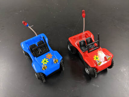
- use the same blue buggy each trial
- start at the same initial position
- use the same track (classroom floor)
Collecting the Data...
1. Start the timer as the person lets go of the buggy from the origin. The front end of the buggy goes behind the initial point before starting.
2. The person with the timer stops the buggy when 5 seconds is up.
3. Measure the distance traveled by the buggy with a meter stick. The distance is from the origin to the front end of the buggy.
4. Record the data (time & distance) on a paper or laptop.
5. Repeat the same steps for different time intervals. Increase the amount of time by 5 seconds. Adjust the interval as needed for a larger range of data. No repeated trials needed.
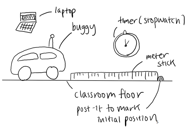
Labeled Diagram
- Let the buggy run for a certain amount of time. After stopping the buggy, measure the total distance traveled by the buggy. Measure the time with a stopwatch, and measure the distance with a meter stick.
- Use the data collected to plot the position-time graph.
1. Start the timer as the person lets go of the buggy from the origin. The front end of the buggy goes behind the initial point before starting.
2. The person with the timer stops the buggy when 5 seconds is up.
3. Measure the distance traveled by the buggy with a meter stick. The distance is from the origin to the front end of the buggy.
4. Record the data (time & distance) on a paper or laptop.
5. Repeat the same steps for different time intervals. Increase the amount of time by 5 seconds. Adjust the interval as needed for a larger range of data. No repeated trials needed.
Labeled Diagram
Recorded Raw Data
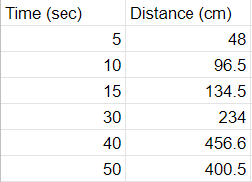
*Uncertainties: Using a stop watch involves a considerable amount of uncertainty since it highly depends on the individual's reaction time.
Graphs & Analysis
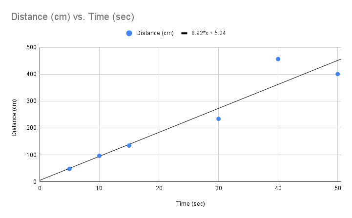
This position graph shows the relationship between time and distance traveled by buggy. The slope is positive, meaning that as time increases, distance increases. Looking at the equation, x = 5.92 t + 5.24, we are able to know that the magnitude of the slope is 8.92. This indicates that position increases by 8.92 cm every second. Since it is a linear model, the change in distance for each and every second is the same. The y-intercept - the position of the buggy when time is zero - is 5.24. Although we started the buggy at the origin, the line of best fit has shifted the y-intercept to 5.24.
Conclusion
According to the data collected from the experiment, time has a linear relationship with the position of the buggy. The slope of the position-time graph is the velocity of the buggy. It indicates the change in the position of the buggy for each second. The equation of the trendline tells us that the steepness of the slope is 8.92, meaning that the distance travelled by the buggy increases by 8.92 cm per second. Since it is a linear model, the slope is constant throughout the graph as 8.92. This suggests that the buggy has a constant velocity of 8.92cm/sec. Moreover, the sign of the slope indicates the direction of the moving object. Since the buggy is starting from the origin and moving forward, the slope is positive.
According to the data collected from the experiment, time has a linear relationship with the position of the buggy. The slope of the position-time graph is the velocity of the buggy. It indicates the change in the position of the buggy for each second. The equation of the trendline tells us that the steepness of the slope is 8.92, meaning that the distance travelled by the buggy increases by 8.92 cm per second. Since it is a linear model, the slope is constant throughout the graph as 8.92. This suggests that the buggy has a constant velocity of 8.92cm/sec. Moreover, the sign of the slope indicates the direction of the moving object. Since the buggy is starting from the origin and moving forward, the slope is positive.
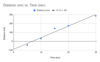
The y-intercept of the graph tells us the initial position of the moving object. Graphically speaking, the y-intercept is the position of the buggy when time equals zero. The y-intercept of the first graph shown above is close to 0, since the initial position was the origin. However, in the position-time graph shown on the left, the y-intercept is close to -100. For this experiment, we repeated the same procedure except having the initial position as -100cm. The vertical shift of the linear model suggests the change in y-intercept.
Through the buggy lab, we figured out the physical interpretation of the slope and the y- intercept of a position-time graph. Using these two elements, we were able to derive a general model for the relationship between position and time.
position = velocity * time + initial position or x final = v * Δt + x initial
This equation can be applied to make a prediction of the position, time, or velocity of the moving object. To solve the unknown, we should know all three other variables.
position = velocity * time + initial position or x final = v * Δt + x initial
This equation can be applied to make a prediction of the position, time, or velocity of the moving object. To solve the unknown, we should know all three other variables.
Evaluation
The most prominent source of uncertainty in this lab was 'judgement error'. The results heavily depended on the individuals' reaction time. The sync between the person who is letting go of the buggy and the person who started the timer might not have been accurate. Also, it was impossible to stop the buggy at exactly 5.00 seconds, since we had to grab the moving object with our hands to make it stop. Different reaction times might have affected the results and the steepness of the graph. Moreover, it was hard to make the buggy travel in a straight line. We had to use multiple meter sticks and place them in a diagonal, assuming the buggy's path to the final position. Although our procedure was theoretically reasonable, it had certain limitations in reality. For improvement, we could have used a buggy with a slower speed so that it is easier to stop the buggy exactly when we need it to stop. We also could have got a wider range of data with a slower buggy, since it would take more time to travel the entire track (classroom floor).
The most prominent source of uncertainty in this lab was 'judgement error'. The results heavily depended on the individuals' reaction time. The sync between the person who is letting go of the buggy and the person who started the timer might not have been accurate. Also, it was impossible to stop the buggy at exactly 5.00 seconds, since we had to grab the moving object with our hands to make it stop. Different reaction times might have affected the results and the steepness of the graph. Moreover, it was hard to make the buggy travel in a straight line. We had to use multiple meter sticks and place them in a diagonal, assuming the buggy's path to the final position. Although our procedure was theoretically reasonable, it had certain limitations in reality. For improvement, we could have used a buggy with a slower speed so that it is easier to stop the buggy exactly when we need it to stop. We also could have got a wider range of data with a slower buggy, since it would take more time to travel the entire track (classroom floor).
