
Independent variable: tangential speed of the bob (m/s)
Dependent variable: acceleration (N/kg)
Controls: radius of the path of the bob (length of string above the rod), mass of the bob
*Controlling the variables - We have to keep the radius of the circular motion constant since the tangential speed of an object, calculated by multiplying angular speed to radius, would be affected by the change in radius. Also, the mass of the bob needs to be the same for each trial because the change in mass would affect the acceleration of the bob.
*Collecting the data - We used a stop watch to measure the time it took for the bob to rotate 20 times, rotating it with different speeds each trial. We also connected a force sensor to the end of the string and connected it to LoggerPro to create a force-time graph each trial. We determined the force of tension by selecting the average force recorded throughout the trial. After collecting the time it took for the bob to rotate 20 times and the net force (force of tension), we calculated the speed and acceleration with the raw data and created a speed - acceleration graph to see the relationship between the two.
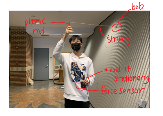
Labeled Diagram
Dependent variable: acceleration (N/kg)
Controls: radius of the path of the bob (length of string above the rod), mass of the bob
*Controlling the variables - We have to keep the radius of the circular motion constant since the tangential speed of an object, calculated by multiplying angular speed to radius, would be affected by the change in radius. Also, the mass of the bob needs to be the same for each trial because the change in mass would affect the acceleration of the bob.
*Collecting the data - We used a stop watch to measure the time it took for the bob to rotate 20 times, rotating it with different speeds each trial. We also connected a force sensor to the end of the string and connected it to LoggerPro to create a force-time graph each trial. We determined the force of tension by selecting the average force recorded throughout the trial. After collecting the time it took for the bob to rotate 20 times and the net force (force of tension), we calculated the speed and acceleration with the raw data and created a speed - acceleration graph to see the relationship between the two.
Labeled Diagram
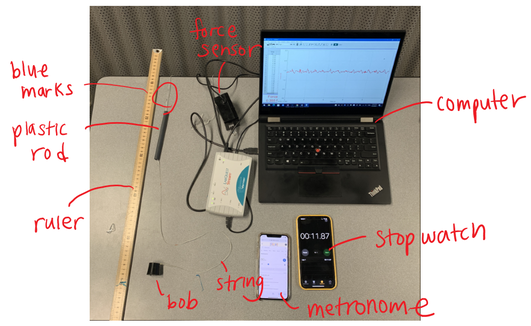
Preparation
1. Measure the mass of the bob
2. Attach the bob to the end of the string and the force sensor to the other end.
3. Use the plastic rod which would help you maintain a constant radius while spinning the bob. Make sure the length of string above the rod is set to a certain length (60cm in our case). Draw marks on the string so that you know that the rod should not fall below it when spinning the bob.
4. Use the metronome to make sure the person is spinning the bob with a constant tempo.
Procedure
1. Hold the force sensor in a stationary position. Start the metronome.
2. Hold the rod and start spinning the bob.
3. When the string becomes parallel to the ground, start the timer. Make sure the person is following the beat of the metronome when spinning the bob.
4. Count 20 rotations and stop the timer.
5. Record the time it took for 20 rotations and the force measurements.
6. Repeat the process with different beats per minute(bpm).
Raw Data
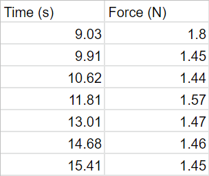
*Possible uncertainties: There is a possibility of judgement errors since we used a stop-watch to measure the time and we had to determine when the bob reached exactly 20 rotations only with our eyes. Also, since we had to select the average force recorded on the time-force graph, there is a possibility of judgement errors.
Processed Data
Processed Data
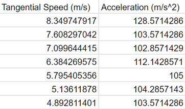
*Tangential speed = angular speed * radius. Therefore, tangential speed = (# of rotations/total time) * 2pi * radius. Since we set the # of rotations to 20 times and the radius to 0.6m, the only unknown variable becomes total time. We insert the raw data for time and calculated the tangential speed.
*Acceleration = net force / mass. Since we know the mass of the bob is 0.014kg, we can substitute the net force (force of tension) for each trial to calculate the acceleration.
Graphical Analysis
*Acceleration = net force / mass. Since we know the mass of the bob is 0.014kg, we can substitute the net force (force of tension) for each trial to calculate the acceleration.
Graphical Analysis
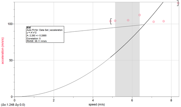
We chose a simple quadratic model (y=Ax^2) as the best fitting curve for the speed-acceleration graph. We initially chose a linear fit, but the negative y-intercept became a problem because an object cannot have a negative non-zero acceleration when its speed is zero. To fix this problem, we tried the proportional fit next. However, although the y-intercept was zero, the graph indicated that the object would have a negative acceleration when the velocity was negative, or, when the bob was spinning in the opposite direction (ex. clockwise to counter clockwise). Negative acceleration suggests that the bob is accelerating away from the center, which isn't true. Although the bob is spinning in the opposite direction, the force of tension would still be towards the center, meaning that acceleration will still be positive. To fulfill these two requirements, we ended up using a simple quadratic model. The y-intercept is 0; acceleration is always positive; and it shows a positive correlation between speed and acceleration. The equation of the graph was "a=2.26v^2". As velocity increases, acceleration increasingly increases.
Conclusion
As the speed of an object in circular motion increases, acceleration increases. The quadratic model we graphed for the speed-acceleration graph indicates that as speed increases, the acceleration increases at a increasing rate. More importantly, through this lab, we were able to derive the formula for Centripetal Acceleration: a = v^2/r (a=centripetal acceleration, v=velocity, r=radius). Centripetal acceleration is an acceleration that points towards the center of rotation, like the spinning bob in our experiment. In other words, the direction of net force is towards the center of rotation. This formula allows us to calculate the tangential acceleration when an object is just changing direction, not speeding up or slowing down. The equation we derived from our experiment was "a=2.26v^2". The constant, 2.26, is supposed to be (1/radius) according to the formula for centripetal acceleration. Since our radius was 0.6m, our constant is supposed to be approximately 1.667, which is quite close to the 2.26 we got. Moreover, through this formula, we are able to connect centripetal acceleration with velocity and acceleration. For example, when the velocity of the object doubles, acceleration quadruples. When the radius is halved, centripetal acceleration is doubled.
Evaluation
I have a medium level of confidence for our lab results. Firstly, as I have mentioned above, there is a possibility of judgement errors when measuring both total time and tension force. This might have affected the processed data for both speed and acceleration. Secondly, we weren't able to collect a wide range of data since if we slowed down the bpm of the metronome, it would be hard to spin the bob in a constant circular path; it would drag downwards and make a smaller circle. To improve, however, we SHOULD collect the larger range of data since the data points we have right now only accounts for the upper points of the quadratic model. Having a wider range of data points would help us find a more accurate best fit curve.
